The increasing depth and size of convolutional neural networks poses a huge challenge for the deployment of deep learning on the mobile side. CNN model compression and acceleration has become one of the research areas that are of great concern to both academia and industry.
Since Alex Net won the ILSVRC 2012 ImageNet Image Classification Competition, the Convolutional Neural Network (CNN) boom has swept the entire computer vision field. The CNN model replaces the traditional hand-crafted features and classifiers, providing not only an end-to-end processing method, but also greatly refreshing the accuracy of each image competition task, and even surpassing the human eye. Accuracy (LFW face recognition task). While CNN models are continually approaching the precision limits of computer vision tasks, their depth and size are also exponentially increasing.
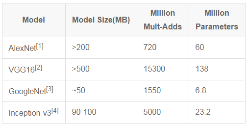
Table 1 Comparison of size, calculation amount and parameter quantity of several classic models
What followed was a very embarrassing scenario: such a huge model could only be used on a limited platform and could not be ported to mobile and embedded chips. Even if you want to transmit over the network, the high bandwidth usage is daunting for many users. On the other hand, large-scale models also pose a huge challenge to device power consumption and operating speed. Therefore, such a model is still some distance away from practical use.
Under such circumstances, the miniaturization and acceleration of the model has become an urgent problem to be solved. In fact, some scholars proposed a series of CNN model compression methods in the early days, including weight prunning and matrix SVD decomposition, but the compression ratio and efficiency are far from satisfactory.
In recent years, algorithms for model miniaturization can be roughly divided into two categories from the perspective of compression: compression from the perspective of model weight values ​​and compression from the perspective of network architecture. On the other hand, from the perspective of balancing the calculation speed, it can be further divided into: only compressing the size and compressing the size while increasing the speed.
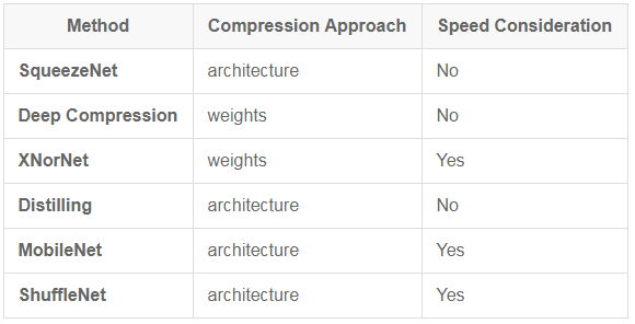
This article focuses on the following representative articles and methods, including SqueezeNet [5], Deep Compression [6], XNorNet [7], Distilling [8], MobileNet [9] and ShuffleNet [10], or as described above. Conduct a general classification:
Table 2 Several classic compression methods and comparison
1.1 Design ideas
SqueezeNet is a miniaturized network model structure proposed by FN Iandola, S. Han et al. in the 2016 paper "SqueezeNet: AlexNet-level accuracy with 50x fewer parameters and < 0.5MB model size". At the same time as the loss accuracy, the original AlexNet was compressed to about 510 times (< 0.5MB).
The core guiding principle of SqueezeNet is to use the fewest parameters while guaranteeing accuracy.
And this is also the ultimate goal of all model compression methods.
Based on this idea, SqueezeNet proposed a 3-point network structure design strategy:
Strategy 1. Replace the 3x3 convolution kernel with a 1x1 convolution kernel.
This strategy is well understood because the parameters of a 1x1 convolution kernel are 1/9 of the 3x3 convolution kernel parameter. This change theoretically compresses the model size by a factor of 9.
Strategy 2. Reduce the number of input channels input to the 3x3 convolution kernel.
We know that for a convolutional layer with a 3x3 convolution kernel, the number of all convolution parameters for that layer (regardless of the offset) is:

Where N is the number of convolution kernels, that is, the number of output channels, and C is the number of input channels.
Therefore, in order to ensure that the network parameters are reduced, it is not only necessary to reduce the number of 3x3 convolution kernels, but also to reduce the number of input channels input to the 3x3 convolution kernel, that is, the number of Cs in the equation.
Strategy 3. Place downsampling as much as possible in the layers behind the network.
In a convolutional neural network, whether the feature map of each layer output is downsampled is determined by the step size of the convolution layer or the pooling layer. An important point is that the higher resolution map (delayed downsampling) can lead to higher classification accuracy, which is intuitively understandable because the higher resolution input can provide The more information there is.
Among the above three strategies, the first two strategies are designed to reduce the number of parameters, and the last one is to maximize network accuracy.
1.2 Network Architecture
Based on the above three strategies, the author proposed a network element structure similar to inception, named fire module. A fire module consists of a squeezed convolutional layer (containing only 1x1 convolution kernels) and an expand convolutional layer (containing 1x1 and 3x3 convolution kernels). Among them, the squeeze layer draws on the idea of ​​inception, using 1x1 convolution kernel to reduce the number of input channels input to the 3x3 convolution kernel in the expand layer. As shown in Figure 1.
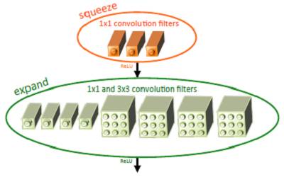
Figure 1 Schematic diagram of the Fire module structure [5]
Among them, the number of 1x1 convolution kernels in the definition of the squeeze layer is s1x1. Similarly, the number of 1x1 convolution kernels in the expand layer is e1x1, and the number of 3x3 convolution kernels is e3x3. Let s1x1 < e1x1 + e3x3 ensure that the number of input channels input to 3x3 is reduced. SqueezeNet's network structure consists of several fire modules, and the article also gives some architectural design details:
To ensure that the 1x1 convolution kernel and the 3x3 convolution kernel have the same size output, the 3x3 convolution kernel uses a 1-pixel zero-padding and step size.
Both the squeeze layer and the expand layer use RELU as the activation function.
50% dropout after fire9
Since the number of parameters of the fully connected layer is huge, the idea of ​​NIN [11] is used to remove the fully connected layer and use global average pooling.
1.3 Experimental results
Table 3 Comparison of different compression methods on ImageNet [5]
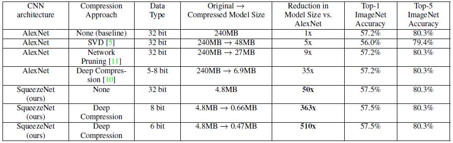
The above table shows that SqueezeNet can achieve the maximum compression ratio without sacrificing accuracy (or even slightly improved) compared to the traditional compression method. The original AlexNet is compressed from 240MB to 4.8MB, and combined with Deep Compression. It can reach 0.47MB, which fully meets the deployment of mobile terminals and the transmission of low bandwidth networks.
In addition, the author also borrowed the ResNet idea, modified the original network structure, added a bypass branch, and improved the classification accuracy by about 3%.
1.4 Speed ​​considerations
Although the article focuses on the size of the compressed model, it is undoubted that SqueezeNet's extensive use of 1x1 and 3x3 convolution kernels in the network structure is conducive to speed improvement. For deep learning frameworks like caffe, convolution In the forward calculation of the layer, the 1x1 convolution kernel can avoid the extra im2col operation, and directly use the gemm for matrix acceleration operation, so the speed optimization has a certain effect. However, the speed-up effect is still limited. In addition, SqueezeNet uses 9 fire modules and two convolutional layers, so a large number of conventional convolution operations are still needed, which is also a bottleneck that affects the speed.
Second, Deep CompressionDeep Compression is from a paper by S. Han 2016 ICLR, "Deep Compression: Compressing Deep Neural Networks with Pruning, Trained Quantization and Huffman Coding." This article won the best paper award of ICLR 2016, and also has a milestone significance, leading the new frenzy of CNN model miniaturization and accelerating research direction, which has brought a lot of excellent work and articles in this field in the past two years. .
2.1 Algorithm flow
Unlike the previous "architecture compression" SqueezeNet, Deep Compression belongs to the "weight compression pie". Both articles are from the S.Han team, so the combination of the two methods, the combination of the two swords, can achieve the ultimate compression effect. The results of this experiment were also verified in the above table.
The algorithm flow of Deep Compression consists of three steps, as shown in Figure 2:
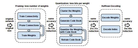
Figure 2 Deep Compression Pipeline [6]
1, Pruning (weight pruning)
The idea of ​​pruning has long been seen in early papers. LeCun et al. used pruning to sparse networks, reducing the risk of overfitting and improving network generalization.
Figure 3 shows the parameter distribution in the LeNet conv1 convolutional layer trained on MNIST. It can be seen that most of the weights are concentrated near 0, and the contribution to the network is small. In the clipping value, the value near 0 is compared. The small weights are set to 0, so that these weights are not activated, so that the remaining non-zero weights are emphasized, and finally the compression size is achieved while ensuring the network accuracy is unchanged.
The experiment found that the model is more sensitive to pruning. Therefore, it is recommended to pruning layer by layer when trimming. In addition, how to automatically select the pruning ratio of each layer is still a subject worthy of further study.
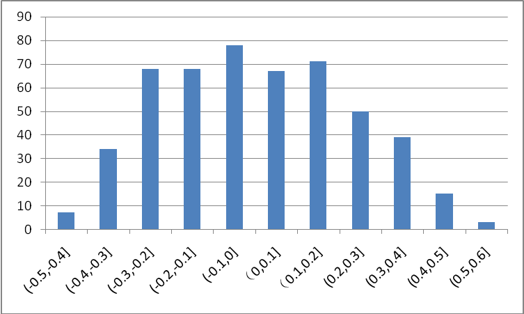
Figure 3 LeNet conv1 layer weight distribution map
2, Quantization (weight quantization)
The weight quantization here is based on weight clustering, which discretizes the weights of the continuous distribution, thereby reducing the number of weights that need to be stored.
Initialize the cluster center, and the experiment proves that the linear initialization effect is the best;
The k-means algorithm is used for clustering, and the weights are divided into different clusters;
In the forward calculation, each weight is represented by its cluster center;
In the backward calculation, the gradient in each cluster is counted and passed back.
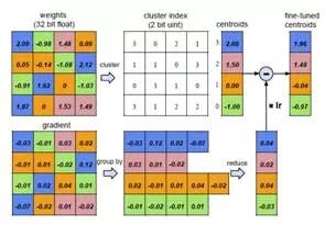
Figure 4 Weight quantization forward and backward calculation process [6]
3, Huffman encoding (Huffman encoding)
Huffman coding uses variable length coding to reduce the average code length and further compress the model size.
2.2 Model storage
The aforementioned pruning and quantification are to achieve a more compact compression of the model to achieve the purpose of reducing the size of the model.
For the model after pruning, since a large number of parameters per layer are 0, it is only necessary to store non-zero values ​​and their subscripts. The article uses CSR (Compressed Sparse Row) for storage. This step can achieve 9x~13x. Compression ratio.
For the quantized model, each weight is represented by its cluster center (for the convolution layer, the cluster center is set to 256, and for the fully connected layer, the cluster center is set to 32), so the corresponding The codebook and subscript greatly reduce the amount of data that needs to be stored. This step can achieve a compression ratio of about 3x.
Finally, the compressed model is further subjected to variable length Huffman coding to achieve a compression ratio of about 1×.
2.3 Experimental results
Table 4 Compression ratios of different networks using Deep Compression [6]
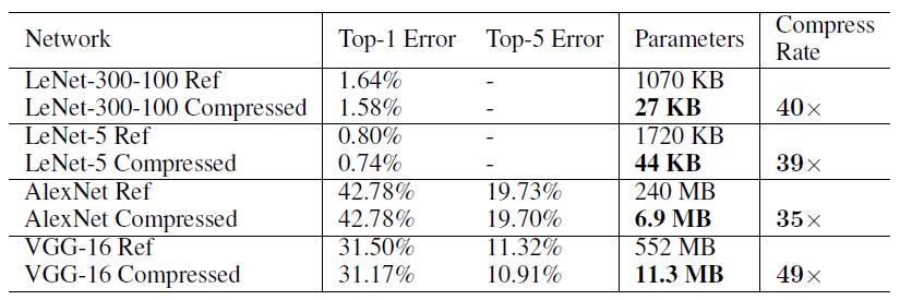
With SqueezeNet+Deep Compression, the original 240M AlexNet can be compressed to 0.47M, achieving a compression ratio of approximately 510x.
2.4 Speed ​​considerations
It can be seen that the main design of Deep Compression is to compress the size of the network storage, but in the forward direction, if the storage model is read into the expansion, it does not bring more speed increase. Therefore, Song H. et al. designed a set of FPGA-based hardware forward acceleration framework EIE [12] for the compressed model. Interested parties can study it.
Third, XNorNetBinary networks have always been one of the long-standing research topics in the field of model compression and acceleration. Compressing the original 32-bit floating-point weight to 1 bit, how to minimize performance loss has become the key to research.
This paper mainly has the following contributions:
A BWN (Binary-Weight-Network) and XNOR-Network are proposed. The former only performs binarization on network parameters, which brings about 32x storage compression and 2x speed improvement, while the latter does two network input and parameters. Valued, with a 58x speed increase while implementing 32x storage compression;
A new algorithm for binarization weights is proposed.
The first to submit a binary network result on a large data set such as ImageNet;
Training from scratch can be achieved without pre-training.
3.1 BWN
In order to train the binary weighted network,  ,among them
 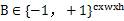 , that is, a binary filter,
  Is the scale factor. By minimizing the objective function, the optimal solution is obtained:

That is, the optimal binarized filter tensor B is the sign function of the original parameters, and the optimal scale factor is the mean of the absolute values ​​of each filter weight.
The training algorithm is shown in Figure 5. It is worth noting that the binarized weights are used only in the forward and backward propagation, and the original parameters are still used when updating the parameters, because if binarization is used The parameters cause a small gradient drop, which makes the training unable to converge.
3.2 XNOR-Net
In XNOR networks, the goal of optimization is to approximate the point multiplication of two real vectors to the point multiplication of two binary vectors, ie  In the formula,
 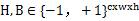 ,
,  Similarly, there is an optimal solution as follows

In convolution calculations, both inputs and weights are quantized to binary values, so traditional multiplication calculations become XOR operations, while non-binarized data calculations account for only a small fraction.
A typical convolution unit in XNOR-Net is shown in Figure 6. Unlike traditional units, the order of each module has been adjusted. In order to reduce the precision loss caused by binarization, the input data is first BN normalized, the BinActiv layer is used to binarize the input, then the binarized convolution operation is performed, and finally the pooling is performed.
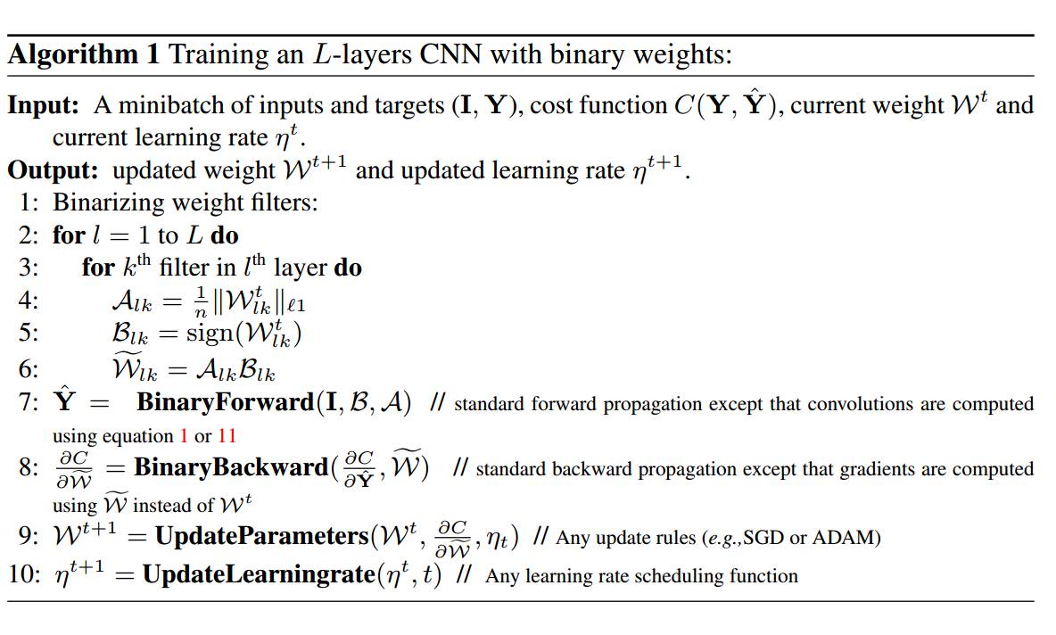
Figure 5 BWN training process [7]
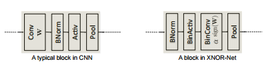
Figure 6 Comparison of traditional convolution units with XNOR-Net convolution units [7]
3.3 Experimental results
Table 5 Comparison of binary networks and AlexNet results on ImageNet [7]
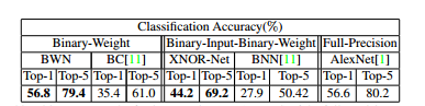
Compared with ALexNet, the BWN network can achieve the same accuracy or even better. XNOR-Net has a lower performance due to binarization of the input.
DistillingThe Distilling algorithm is a network migration-like learning algorithm proposed by Hinton et al. in the paper Distillering the Knowledge in a Neural Network.
4.1 Basic ideas
Distilling literally translates into distillation. The basic idea is to teach small network learning through a large network with good performance, so that small networks can have the same performance as large networks, but the scale of small network parameters after distillation is much smaller than the original large network. In order to achieve the purpose of compressing the network.
Among them, the objective function of the trained model consists of two parts.
1) Cross entropy with the softmax output of the cumbersome model, called soft target. Among them, the calculation of softmax adds the super-parameter temperature T to control the output, and the calculation formula becomes
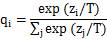
The larger the temperature T is, the more moderate the distribution of the output is. The smaller the probability zi/T is, the larger the entropy is. However, if T is too large, the uncertainty caused by larger entropy increases, and the indistinguishability is increased.
As for why the soft target is used to calculate the loss, the author believes that in the classification problem, the groundtruth is a certainty, that is, one-hot vector. In terms of handwritten digit classification, for a number 3, the probability that its label is 3 is 1, but the probability of other values ​​is 0, and for soft target, it can represent the probability that label is 3, if this number is written Like 5, you can also give a certain probability that the label is 5, thus providing more information, such as
2) Cross entropy with true value (groundtruth) (T=1)
The loss of training is the weighted sum of the above two losses, usually the second item is much smaller.
4.2 Experimental results
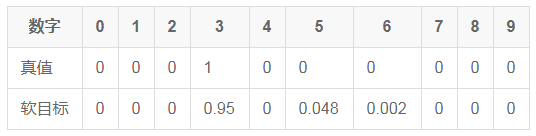
The author gives a comparison of experimental results on speech recognition, as shown in the following table.
Table 6 Accuracy comparison between distillation model and original model [8]
The above table shows that the accuracy of the model after distillation and the error rate of the single word are comparable to those of the 10 models used to generate the soft target. The small model successfully learned the recognition ability of the large model.
4.3 Speed ​​considerations
The introduction of Distilling was not originally aimed at network acceleration, and the efficiency of the final calculation still depends on the calculation scale of the distillation model. However, theoretically, the calculation speed of the distilled small model relative to the original large model will be improved to a certain extent, but the speed is improved. The trade-off between ratio and performance maintenance is a direction worth studying.
Five, MobileNetMobileNet is a lightweight network architecture proposed by Google for mobile deployment. Considering the limited computing resources on the mobile side and the stringent speed requirements, MobileNet introduces the group idea originally used in traditional networks, that is, the convolution calculation of the limit filter is only for the input in a specific group, thus greatly reducing the convolution calculation. The amount increases the speed of the forward calculation of the mobile terminal.
5.1 Volume Integration Solution
MobileNet draws on the idea of ​​factorized convolution to divide the ordinary convolution operation into two parts:
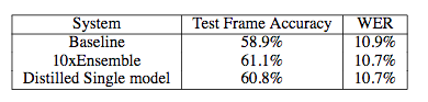
Depthwise Convolution
Each convolution kernel filter only performs a convolution operation on a specific input channel, as shown in the following figure, where M is the number of input channels and DK is the convolution kernel size:
Figure 7 Depthwise Convolution [9]
The computational complexity of Depthwise convolution is DKDKMDFDF, where DF is the size of the feature map of the convolutional layer output.
Pointwise Convolution
A multi-channel output of the depthwise convolution layer is combined using a 1x1 convolution kernel, as shown in the following figure, where N is the number of output channels:
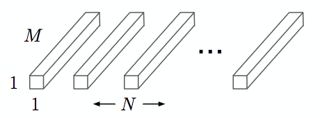
Figure 8 Pointwise Convolution[9]
The computational complexity of Pointwise Convolution is MNDFDF
The above two steps are collectively called depthwise separable convolution
The computational complexity of standard convolution operations is DKDKMNDFDF
Therefore, by decomposing the standard volume integral into a two-layer convolution operation, the theoretical computational efficiency improvement ratio can be calculated:
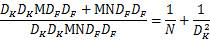
For a 3x3 size convolution kernel, the depthwise separable convolution can theoretically bring about an 8 to 9 times efficiency improvement.
5.2 Model Architecture
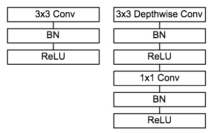
Figure 9 Comparison of a common convolution unit with a MobileNet convolution unit [9]
MobileNet's convolution unit is shown in the figure above, followed by a BN operation and a ReLU operation after each convolution operation. In MobileNet, since the 3x3 convolution kernel is only used in depthwise convolution, 95% of the computation is concentrated in the 1x1 convolution in pointwise convolution. For caffe and other deep learning frameworks that use the matrix operation GEMM to achieve convolution, the 1x1 convolution does not need to perform the im2col operation, so the matrix operation acceleration library can be directly used for fast calculation, thereby improving the calculation efficiency.
5.3 Experimental results
Table 7 Accuracy comparison between MobileNet and mainstream large models on ImageNet [9]
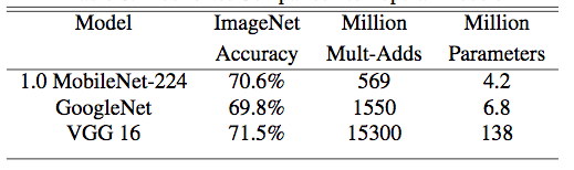
The above table shows that MobileNet can effectively reduce the number of calculation operations and the amount of parameters while ensuring the same accuracy, making real-time forward calculation on the mobile side possible.
Six, ShuffleNetShuffleNet is a network architecture that Face++ proposed for mobile forward deployment this year. ShuffleNet is based on MobileNet's group idea, which limits convolution operations to specific input channels. In contrast, ShuffleNet breaks up the input group, ensuring that the receptive field of each convolution kernel can be distributed to different group inputs, increasing the learning ability of the model.
6.1 Design ideas
We know that group operations in convolution can greatly reduce the number of calculations for convolution operations, and this change brings speed gain and performance maintenance to be verified in articles such as MobileNet. However, another problem brought by the group operation is that the specific filter only works on the input of a specific channel, which hinders the flow of information between the channels. The more the number of groups, the richer the information that can be encoded. However, the number of input channels per group is reduced, which may cause degradation of a single convolution filter, which weakens the network's expressive ability to some extent.
6.2 Network Architecture
In this work, the design of the network architecture mainly has the following innovations:
Proposed a BottleNeck unit similar to ResNet
Drawing on ResNet's bypass branch idea, ShuffleNet also introduced similar network elements. The difference is that in the stride=2 unit, the concat operation replaces the add operation, and the average pooling is used instead of the 1x1stride=2 convolution operation, which effectively reduces the amount of calculation and parameters. The unit structure is shown in Figure 10.
It is proposed that using 1x1 convolution in group operation will result in better classification performance.
As mentioned in MobileNet, the 1x1 convolution operation accounts for about 95% of the computation, so the author changed 1x1 to group convolution, which greatly reduced the computational load compared to MobileNet.
It is proposed that the core shuffle operation breaks up the channels in different groups to ensure the information transmission between different input channels.
ShuffleNet's shuffle operation is shown in Figure 11.
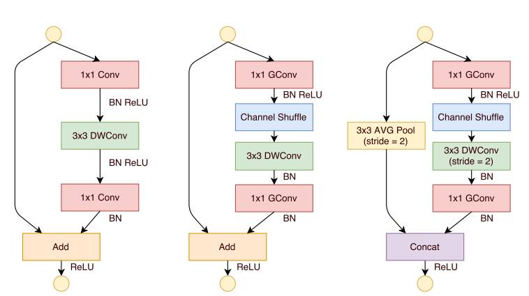
Figure 10 ShuffleNet network unit [10]
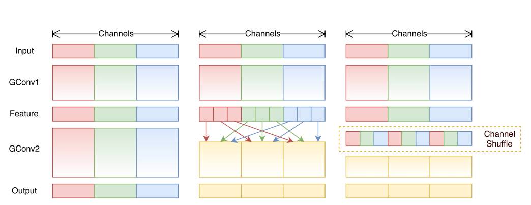
Figure 11 shuffle operation between different groups [10]
6.3 Experimental results
Table 8 Accuracy comparison between ShuffleNet and MobileNet on ImageNet [10]
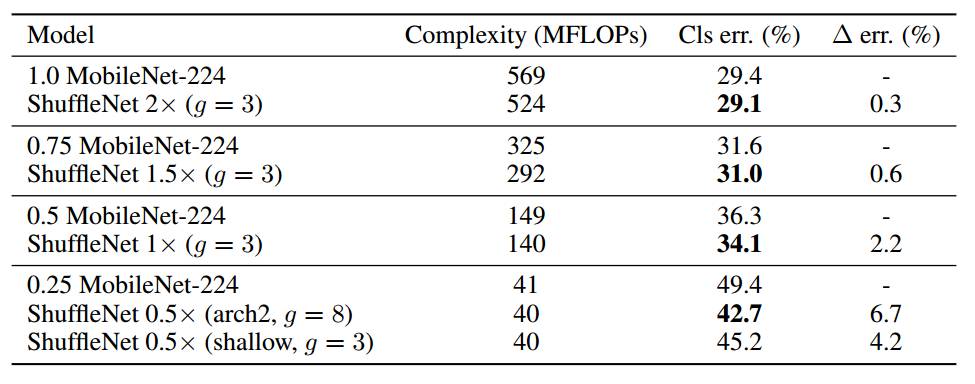
The above table shows that compared to MobileNet, the forward calculation of ShuffleNet has not only been effectively reduced, but also the classification error rate has been significantly improved, which verifies the feasibility of the network.
6.4 Speed ​​considerations
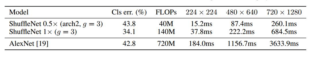
The author verified the network efficiency on the ARM platform. Given the factors such as memory reading and thread scheduling, the author found that the theoretical 4x speed increase corresponds to about 2.6x in actual deployment. The author gives a comparison of the speed of the original AlexNet, as shown in the following table.
Table 9 Speed ​​comparison between ShuffleNet and AlexNet on ARM platform [10]
Conclusion
In recent years, in addition to the acceleration of many CNN models emerging in the academic world, major companies in the industry have also launched their own mobile forward computing framework, such as Google's Tensorflow, Facebook's caffe2 and Apple's CoreML just launched this year. It is believed that the combination of continuous iterative optimization of network architecture and evolving hardware computing acceleration technology, the deployment of deep learning in the future will not be a problem.
references
[1] ImageNet Classification with Deep Convolutional Neural Networks
[2] Very Deep Convolutional Networks for Large-Scale Image Recognition
[3] Going Deeper with Convolutions
[4] Rethinking the Inception Architecture for Computer Vision
[5] SqueezeNet: AlexNet-level accuracy with 50x fewer parameters and < 0.5MB model size
[6] Deep Compression: Compressing Deep Neural Networks with Pruning, Trained Quantization and Huffman Coding
[7] Distilling the Knowledge in a Neural Network
[8] XNOR-Net: ImageNet Classification Using Binary Convolutional Neural Networks
[9] MobileNets: Efficient Convolutional Neural Networks for Mobile Vision Applications
[10] ShuffleNet: An Extremely Efficient Convolutional Neural Network for Mobile Devices
[11] Network in Network
[12] EIE: Efficient Inference Engine on Compressed Deep Neural Network
With the improvement of people's living standards, most of the residents will go to the supermarket to buy things, which has led to the popularity of supermarkets, and the popularity of supermarkets has also led to the development of supermarket shelves.
The main purpose of supermarket shelves is to place and display goods, but also to store goods. They have the characteristics of simple installation and easy operation, and have been widely used in various supermarkets.
The types of supermarket shelves are as follows:
1. Large supermarket shelves:
Hypermarkets have rich displays of goods, so they have higher requirements for shelf load-bearing. Its main customers are those of national hypermarkets.
2. Standard supermarket shelves:
Standard supermarket shelves are specially developed and designed for standard supermarkets. The biggest feature is lightness and beauty. It does not have the complex types of accessories like supermarket shelves, and the display method has also been adjusted accordingly, paying more attention to the display effect of goods and humanized display. Its main customers are local chain-sized medium-sized supermarkets.
3. Convenience store shelves:
Convenience store shelves are suitable for convenience stores and drugstores. They adopt the concept of tool-free installation and are easy to install. The biggest feature of the shelf is exquisite, light, beautiful, and strong specialization. Its main customers such as: 7-11 and so on.
Supermarket Shelves,Double Side Supermarket Shelves,Supermarket Storage Shelves,Multi-Layer Supermarket Shelves
Wuxi Lerin New Energy Technology Co.,Ltd. , https://www.lerin-tech.com